The 68% Rule

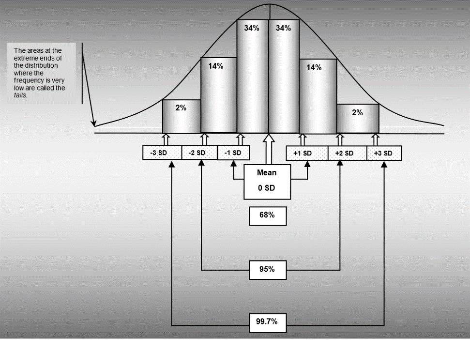
Diving into statistics often feels like embarking on a thrilling quest filled with nuances, insights, and intriguing patterns. Among the key aspects that statisticians, students, and data enthusiasts encounter on this journey is the concept of standard deviation—a measure that, at its core, defines the spread of a dataset. When paired with the iconic bell-shaped normal distribution, standard deviation unravels a principle so foundational that it deserves its spotlight: The 68% Rule. Let’s delve deep into this rule and grasp its significance.

A Refresher: The Role of Standard Deviation

Before we tackle the 68% Rule, let’s briefly revisit the concept of standard deviation. It represents the average distance of individual scores or data points from the mean (or average) of a distribution. In layman’s terms, standard deviation gives us a sense of how spread out or clustered the data points are around the mean. If the standard deviation is low, it indicates that the data points are relatively close to the mean; conversely, a high standard deviation suggests a wider spread.

Now, armed with an understanding of standard deviation, imagine being able to gauge how “typical” or “extreme” a particular score is. By examining the difference between an individual’s score and the mean, and then relating this difference to the standard deviation, we can determine just that!

The Heart of the Matter: Introducing the 68% Rule

One of the defining characteristics of the normal distribution—our symmetrical, bell-shaped curve—is the predictability of data spread in relation to standard deviations. This brings us to the revered 68% Rule.

In essence, the rule articulates that approximately 68% of the data points (or cases) in a normal distribution fall within one standard deviation unit from the mean. This includes both the left and the right sides of the mean, ensuring that our data’s symmetry is maintained.

To clarify, consider the following hypothetical:

Imagine a standardized test where the mean score is 100, and the standard deviation is 10. According to the 68% Rule, we can predict that about 68% of the students who take this test will score between 90 (which is one standard deviation below the mean) and 110 (one standard deviation above the mean). So, if you’re a student who scored 105, you’re well within the “typical” range for this test!

When Does the 68% Rule Apply?

It’s essential to approach this rule with a discerning eye. While it’s a foundational concept for normal distributions, its applicability diminishes as we deviate from the bell curve. That’s right—the 68% Rule is most accurate for perfectly normal distributions. As the shape of the distribution starts to differ from the iconic bell shape, our trusty rule’s precision diminishes.

Therefore, it’s paramount to ensure that your dataset approximates a normal distribution before making predictions or inferences based on the 68% Rule. Otherwise, you risk drawing misleading conclusions.

Visualizing the 68% Rule: Areas Under the Normal Curve

Visual learners, rejoice! The beauty of the 68% Rule (and other rules related to standard deviations in a normal distribution) is that it can be visualized and conceptualized with the help of the areas under the curve.

When you look at the bell curve representing a normal distribution, imagine shading the area that falls within one standard deviation from the mean. This shaded region, encompassing the bulging center of our bell, represents the 68% of data points. It provides a tangible representation of the majority of scores that cluster around the average, allowing for intuitive understanding and interpretation.

---

Conclusion

The 68% Rule offers a fascinating glimpse into the predictability inherent in the normal distribution. As you journey further into the world of statistics, such foundational principles will become stepping stones, enabling you to unlock more complex insights and analyses. Always remember, though, to approach each rule with critical thinking, ensuring that your data aligns with the assumptions before drawing any conclusions.

Summary

Ever noticed how scores or measurements often cluster around an average? In the world of statistics, the spread of these scores is measured by something called the “standard deviation.” When we delve into a particular kind of data pattern called the “normal distribution” (which looks like a bell curve), we stumble upon a cool rule. This is the 68% Rule.

Simply put, in a bell-shaped data pattern, about 68% of all scores will be close to the average, falling within a range defined by the standard deviation. For instance, if students take a test with an average score of 100 and a standard deviation of 10, we can guess that around 68% of students will score between 90 and 110.

However, a key thing to remember is this rule is best for perfect bell-shaped patterns. If our data doesn’t quite look like a bell, the rule might not be as precise. So, always be sure your data fits the bell shape before using the 68% Rule. In short, this rule helps us understand where most scores in a dataset are likely to lie!

[ Back | Contents | Next ]

Last Modified:  10/16/2023